Enterprise Edition
Timefold Solver Enterprise Edition is a commercial product that offers additional features, such as nearby selection and multi-threaded solving. These features are essential to scale out to huge datasets.
Unlike Timefold Solver Community Edition, the Enterprise Edition is not open-source. We offer free licenses to non-profit organizations and for academic research. Everyone else may be entitled to a trial license to evaluate the product before purchasing. Please contact Timefold to obtain an Enterprise license.
| Looking for quicker time-to-value? Timefold offers pre-built, fully tuned optimization models, no constraint building required. Just plug into our API and start optimizing immediately. |
For a high-level overview of the differences between Timefold offerings, see Timefold Pricing.
1. Switch to Enterprise Edition
To switch from Timefold Solver Community Edition to Enterprise Edition,
contact us first to obtain an Enterprise License.
This license is represented by a file named timefold-enterprise-license.pem,
which you can introduce to your project by one of the following methods:
-
Store the license’s PEM string in the
TIMEFOLD_ENTERPRISE_LICENSEenvironment variable. -
Store the absolute path to the file in
TIMEFOLD_ENTERPRISE_LICENSE_PATHenvironment variable. -
Place the file in the user’s home directory.
-
Place the file in the root of your application classpath.
Having done that, replace references to Community Edition artifacts by their Enterprise Edition counterparts as shown in the following table:
| Community Edition | Enterprise Edition |
|---|---|
|
|
|
|
|
|
|
|
2. Features of Enterprise Edition
The following features are only available in Timefold Solver Enterprise Edition:
2.1. Nearby selection
|
This feature is a commercial feature of Timefold Solver Enterprise Edition. It is not available in the Community Edition. |
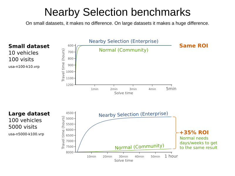
In some use cases (such as TSP and VRP, but also in other cases), changing entities to nearby values or swapping nearby entities leads to better results faster.
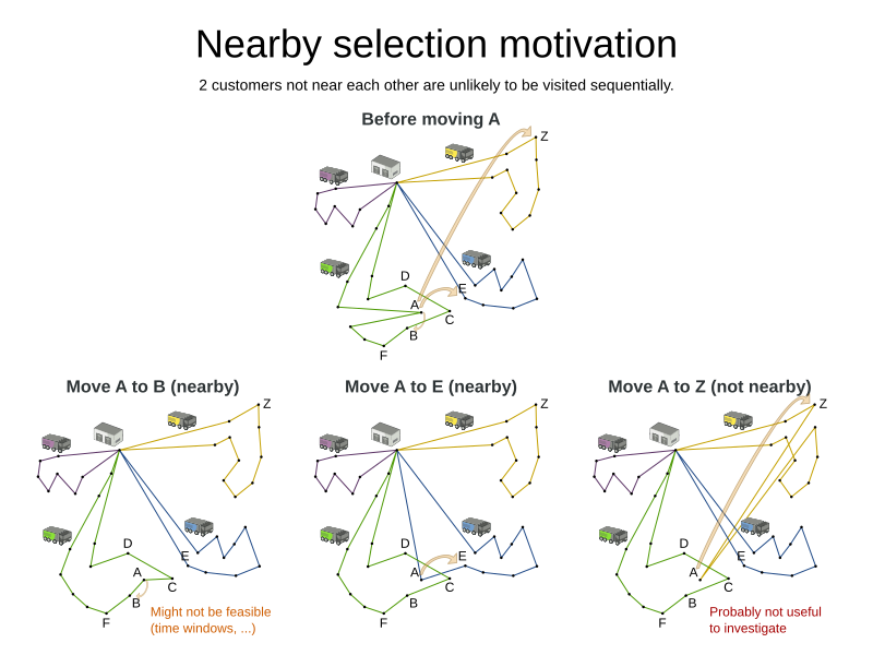
This can heavily increase scalability and improve solution quality:
Nearby selection increases the probability of selecting an entity or value which is nearby to the first entity being moved in that move.
The distance between two entities or values is domain specific.
Therefore, implement the NearbyDistanceMeter interface:
-
Java
public interface NearbyDistanceMeter<Origin_, Desination_> {

    double getNearbyDistance(Origin_ origin, Destination_ destination);

}
In a nutshell, when nearby selection is used in a list move selector,
Origin_ is always a planning value (for example Customer)
but Destination_ can be either a planning value or a planning entity.
That means that in VRP the distance meter must be able to handle both Customer and Vehicle as the Destination_ argument:
-
Java
public class CustomerNearbyDistanceMeter implements NearbyDistanceMeter<Customer, LocationAware> {

    public double getNearbyDistance(Customer origin, LocationAware destination) {
        return origin.getDistanceTo(destination);
    }

}|
The Nearby configuration is not enabled for the Construction Heuristics because the method will analyze all possible moves. Adding Nearby in this situation would only result in unnecessary costs involving the generation of the distance matrix and sorting operations without taking advantage of the feature. |
2.1.1. Nearby selection with a list variable
To quickly configure nearby selection with a planning list variable,
add nearbyDistanceMeterClass element to your configuration file.
The following enables nearby selection with a list variable
for the local search:
<?xml version="1.0" encoding="UTF-8"?>
<solver xmlns="https://timefold.ai/xsd/solver">
    ...
    <nearbyDistanceMeterClass>org.acme.vehiclerouting.domain.solver.nearby.CustomerNearbyDistanceMeter</nearbyDistanceMeterClass>
    ...
</solver>
By default, the following move selectors are included: Change, Swap, Change with Nearby, Swap with Nearby, and 2-OPT with Nearby.
Advanced configuration for local search
To customize the move selectors,
add a nearbySelection element in the destinationSelector, valueSelector or subListSelector
and use mimic selection
to specify which destination, value, or subList should be nearby the selection.
    <unionMoveSelector>
      <listChangeMoveSelector>
        <valueSelector id="valueSelector1"/>
        <destinationSelector>
          <nearbySelection>
            <originValueSelector mimicSelectorRef="valueSelector1"/>
            <nearbyDistanceMeterClass>org.acme.vehiclerouting.domain.solver.nearby.CustomerNearbyDistanceMeter</nearbyDistanceMeterClass>
          </nearbySelection>
        </destinationSelector>
      </listChangeMoveSelector>
      <listSwapMoveSelector>
        <valueSelector id="valueSelector2"/>
        <secondaryValueSelector>
          <nearbySelection>
            <originValueSelector mimicSelectorRef="valueSelector2"/>
            <nearbyDistanceMeterClass>org.acme.vehiclerouting.domain.solver.nearby.CustomerNearbyDistanceMeter</nearbyDistanceMeterClass>
          </nearbySelection>
        </secondaryValueSelector>
      </listSwapMoveSelector>
      <subListChangeMoveSelector>
        <selectReversingMoveToo>true</selectReversingMoveToo>
        <subListSelector id="subListSelector3"/>
        <destinationSelector>
          <nearbySelection>
            <originSubListSelector mimicSelectorRef="subListSelector3"/>
            <nearbyDistanceMeterClass>org.acme.vehiclerouting.domain.solver.nearby.CustomerNearbyDistanceMeter</nearbyDistanceMeterClass>
          </nearbySelection>
        </destinationSelector>
      </subListChangeMoveSelector>
      <subListSwapMoveSelector>
        <selectReversingMoveToo>true</selectReversingMoveToo>
        <subListSelector id="subListSelector4"/>
        <secondarySubListSelector>
          <nearbySelection>
            <originSubListSelector mimicSelectorRef="subListSelector4"/>
            <nearbyDistanceMeterClass>org.acme.vehiclerouting.domain.solver.nearby.CustomerNearbyDistanceMeter</nearbyDistanceMeterClass>
          </nearbySelection>
        </secondarySubListSelector>
      </subListSwapMoveSelector>
    </unionMoveSelector>
2.1.2. Power-tweaking distribution type
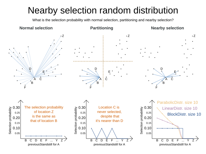
The solver allows you to tweak the distribution type of the nearby selection, or how likely are the nearest elements to be selected based on their distance from the current.
|
Only tweak the default settings if you are prepared to back your choices by extensive benchmarking. |
The following NearbySelectionDistributionTypes are supported:
-
PARABOLIC_DISTRIBUTION(default): Nearest elements are selected with a higher probability.<nearbySelection> <parabolicDistributionSizeMaximum>80</parabolicDistributionSizeMaximum> </nearbySelection>A
distributionSizeMaximumparameter should not be 1 because if the nearest is already the planning value of the current entity, then the only move that is selectable is not doable. To allow every element to be selected regardless of the number of entities, only set the distribution type (so without adistributionSizeMaximumparameter):<nearbySelection> <nearbySelectionDistributionType>PARABOLIC_DISTRIBUTION</nearbySelectionDistributionType> </nearbySelection> -
BLOCK_DISTRIBUTION: Only the n nearest are selected, with an equal probability. For example, select the 20 nearest:<nearbySelection> <blockDistributionSizeMaximum>20</blockDistributionSizeMaximum> </nearbySelection> -
LINEAR_DISTRIBUTION: Nearest elements are selected with a higher probability. The probability decreases linearly.<nearbySelection> <linearDistributionSizeMaximum>40</linearDistributionSizeMaximum> </nearbySelection> -
BETA_DISTRIBUTION: Selection according to a beta distribution. Slows down the solver significantly.<nearbySelection> <betaDistributionAlpha>1</betaDistributionAlpha> <betaDistributionBeta>5</betaDistributionBeta> </nearbySelection>
2.2. Multi-threaded solving
Multi-threaded solving is a term which encapsulates several features that allow Timefold Solver to run on multi-core machines. Timefold Solver Enterprise Edition makes multi-threaded solving more powerful by introducing multi-threaded incremental solving and partitioned search.
For a primer on multi-threaded solving in general, see Multi-threaded solving.
2.2.1. Multi-threaded incremental solving
|
This feature is a commercial feature of Timefold Solver Enterprise Edition. It is not available in the Community Edition. |
With this feature, the solver can run significantly faster, getting you the right solution earlier. It has been designed to speed up the solver in cases where move evaluation is the bottleneck. This typically happens when the constraints are computationally expensive, or when the dataset is large.
-
The sweet spot for this feature is when the move evaluation speed is up to 10 thousand per second. In this case, we have observed the algorithm to scale linearly with the number of move threads. Every additional move thread will bring a speedup, albeit with diminishing returns.
-
For move evaluation speeds on the order of 100 thousand per second, the algorithm no longer scales linearly, but using 4 to 8 move threads may still be beneficial.
-
For even higher move evaluation speeds, the feature does not bring any benefit. At these speeds, move evaluation is no longer the bottleneck. If the solver continues to underperform, perhaps you’re suffering from score traps or you may benefit from custom moves to help the solver escape local optima.
|
These guidelines are strongly dependent on move selector configuration, size of the dataset and performance of individual constraints. We recommend you benchmark your use case to determine the optimal number of move threads for your problem. |
Enabling multi-threaded incremental solving
Enable multi-threaded incremental solving
by adding a @PlanningId annotation
on every planning entity class and planning value class.
Then configure a moveThreadCount:
-
Quarkus
-
Spring
-
Java
-
XML
Add the following to your application.properties:
quarkus.timefold.solver.move-thread-count=AUTOAdd the following to your application.properties:
timefold.solver.move-thread-count=AUTOUse the SolverConfig class:
SolverConfig solverConfig = new SolverConfig()
    ...
    .withMoveThreadCount("AUTO");
Add the following to your solverConfig.xml:
<solver xmlns="https://timefold.ai/xsd/solver" xmlns:xsi="http://www.w3.org/2001/XMLSchema-instance"
xsi:schemaLocation="https://timefold.ai/xsd/solver https://timefold.ai/xsd/solver/solver.xsd">

    ...
    <moveThreadCount>AUTO</moveThreadCount>
    ...

</solver>
Setting moveThreadCount to AUTO allows Timefold Solver to decide how many move threads to run in parallel.
This formula is based on experience and does not hog all CPU cores on a multi-core machine.
A moveThreadCount of 4 saturates almost 5 CPU cores.
the 4 move threads fill up 4 CPU cores completely
and the solver thread uses most of another CPU core.
The following moveThreadCounts are supported:
-
NONE(default): Don’t run any move threads. Use the single threaded code. -
AUTO: Let Timefold Solver decide how many move threads to run in parallel. On machines or containers with little or no CPUs, this falls back to the single threaded code. -
Static number: The number of move threads to run in parallel.
It is counter-effective to set a moveThreadCount
that is higher than the number of available CPU cores,
as that will slow down the move evaluation speed.
|
In cloud environments where resource use is billed by the hour, consider the trade-off between cost of the extra CPU cores needed and the time saved. Compute nodes with higher CPU core counts are typically more expensive to run and therefore you may end up paying more for the same result, even though the actual compute time needed will be less. |
|
Multi-threaded solving is still reproducible, as long as the resolved |
Advanced configuration
There are additional parameters you can supply to your solverConfig.xml:
<solver xmlns="https://timefold.ai/xsd/solver" xmlns:xsi="http://www.w3.org/2001/XMLSchema-instance"
    xsi:schemaLocation="https://timefold.ai/xsd/solver https://timefold.ai/xsd/solver/solver.xsd">
  <moveThreadCount>4</moveThreadCount>
  <threadFactoryClass>...MyAppServerThreadFactory</threadFactoryClass>
  ...
</solver>
To run in an environment that doesn’t like arbitrary thread creation,
use threadFactoryClass to plug in a custom thread factory.
2.2.2. Partitioned search
|
This feature is a commercial feature of Timefold Solver Enterprise Edition. It is not available in the Community Edition. |
Algorithm description
It is often more efficient to partition large data sets (usually above 5000 planning entities) into smaller pieces and solve them separately. Partition Search is multi-threaded, so it provides a performance boost on multi-core machines due to higher CPU utilization. Additionally, even when only using one CPU, it finds an initial solution faster, because the search space sum of a partitioned Construction Heuristic is far less than its non-partitioned variant.
However, partitioning does lead to suboptimal results, even if the pieces are solved optimally, as shown below:
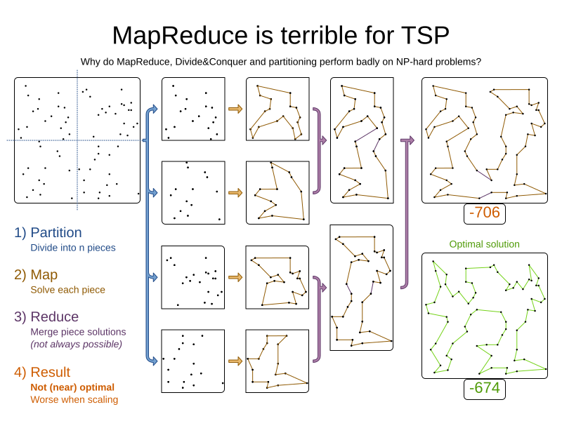
It effectively trades a short term gain in solution quality for long term loss. One way to compensate for this loss, is to run a non-partitioned Local Search after the Partitioned Search phase.
|
Not all use cases can be partitioned. Partitioning only works for use cases where the planning entities and value ranges can be split into n partitions, without any of the constraints crossing boundaries between partitions. |
Configuration
Simplest configuration:
  <partitionedSearch>
    <solutionPartitionerClass>...MyPartitioner</solutionPartitionerClass>
  </partitionedSearch>
Also add a @PlanningId annotation
on every planning entity class and planning value class.
There are several ways to partition a solution.
Advanced configuration:
  <partitionedSearch>
    ...
    <solutionPartitionerClass>...MyPartitioner</solutionPartitionerClass>
    <runnablePartThreadLimit>4</runnablePartThreadLimit>

    <constructionHeuristic>...</constructionHeuristic>
    <localSearch>...</localSearch>
  </partitionedSearch>
The runnablePartThreadLimit allows limiting CPU usage to avoid hanging your machine, see below.
To run in an environment that doesn’t like arbitrary thread creation, plug in a custom thread factory.
|
A logging level of |
Just like a <solver> element,
the <partitionedSearch> element can contain one or more phases.
Each of those phases will be run on each partition.
A common configuration is to first run a Partitioned Search phase (which includes a Construction Heuristic and a Local Search) followed by a non-partitioned Local Search phase:
  <partitionedSearch>
    <solutionPartitionerClass>...MyPartitioner</solutionPartitionerClass>

    <constructionHeuristic/>
    <localSearch>
      <termination>
        <diminishedReturns />
      </termination>
    </localSearch>
  </partitionedSearch>
  <localSearch/>
Partitioning a solution
Custom SolutionPartitioner
To use a custom SolutionPartitioner, configure one on the Partitioned Search phase:
  <partitionedSearch>
    <solutionPartitionerClass>...MyPartitioner</solutionPartitionerClass>
  </partitionedSearch>
Implement the SolutionPartitioner interface:
public interface SolutionPartitioner<Solution_> {

    List<Solution_> splitWorkingSolution(Solution_ workingSolution, Integer runnablePartThreadLimit);

}
The size() of the returned List is the partCount (the number of partitions).
This can be decided dynamically, for example, based on the size of the non-partitioned solution.
The partCount is unrelated to the runnablePartThreadLimit.
To configure values of a SolutionPartitioner dynamically in the solver configuration
(so the Benchmarker can tweak those parameters),
add the solutionPartitionerCustomProperties element and use custom properties:
<partitionedSearch>
<solutionPartitionerClass>...MyPartitioner</solutionPartitionerClass>
<solutionPartitionerCustomProperties>
<property name="myPartCount" value="8"/>
<property name="myMinimumProcessListSize" value="100"/>
</solutionPartitionerCustomProperties>
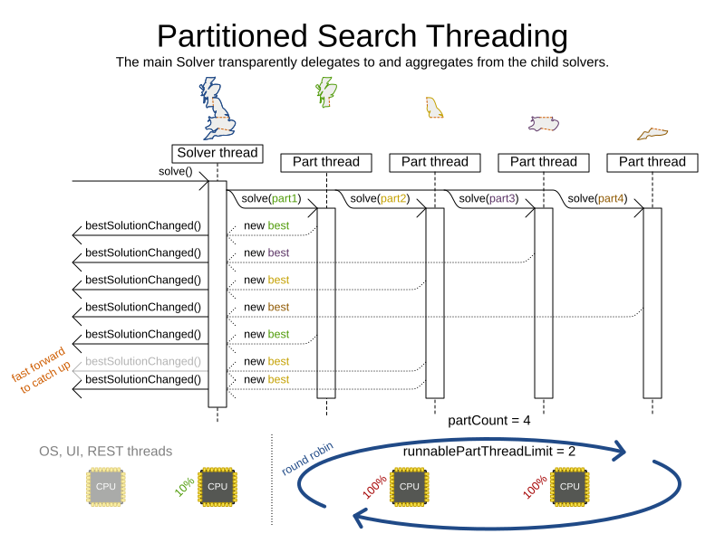
</partitionedSearch>Runnable part thread limit
When running a multi-threaded solver, such as Partitioned Search, CPU power can quickly become a scarce resource, which can cause other processes or threads to hang or freeze. However, Timefold Solver has a system to prevent CPU starving of other processes (such as an SSH connection in production or your IDE in development) or other threads (such as the servlet threads that handle REST requests).
As explained in sizing hardware and software,
each solver (including each child solver) does no IO during solve() and therefore saturates one CPU core completely.
In Partitioned Search, every partition always has its own thread, called a part thread.
It is impossible for two partitions to share a thread,
because of asynchronous termination:
the second thread would never run.
Every part thread will try to consume one CPU core entirely, so if there are more partitions than CPU cores,
this will probably hang the system.
Thread.setPriority() is often too weak to solve this hogging problem, so another approach is used.
The runnablePartThreadLimit parameter specifies how many part threads are runnable at the same time.
The other part threads will temporarily block and therefore will not consume any CPU power.
This parameter basically specifies how many CPU cores are donated to Timefold Solver.
All part threads share the CPU cores in a round-robin manner
to consume (more or less) the same number of CPU cycles:
The following runnablePartThreadLimit options are supported:
-
UNLIMITED: Allow Timefold Solver to occupy all CPU cores, do not avoid hogging. Useful if a no hogging CPU policy is configured on the OS level. -
AUTO(default): Let Timefold Solver decide how many CPU cores to occupy. This formula is based on experience. It does not hog all CPU cores on a multi-core machine. -
Static number: The number of CPU cores to consume. For example:
<runnablePartThreadLimit>2</runnablePartThreadLimit>
|
If the |
2.2.3. Custom thread factory (WildFly, GAE, …)
The threadFactoryClass allows to plug in a custom ThreadFactory for environments
where arbitrary thread creation should be avoided,
such as most application servers (including WildFly) or Google App Engine.
Configure the ThreadFactory on the solver to create the move threads
and the Partition Search threads with it:
<solver xmlns="https://timefold.ai/xsd/solver" xmlns:xsi="http://www.w3.org/2001/XMLSchema-instance"
    xsi:schemaLocation="https://timefold.ai/xsd/solver https://timefold.ai/xsd/solver/solver.xsd">
  <threadFactoryClass>...MyAppServerThreadFactory</threadFactoryClass>
  ...
</solver>
2.3. Automatic node sharing
|
This feature is a commercial feature of Timefold Solver Enterprise Edition. It is not available in the Community Edition. |
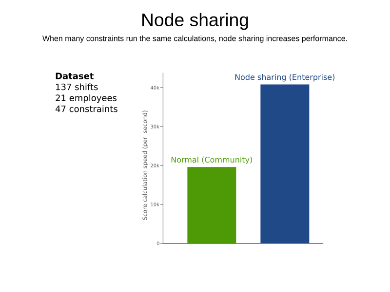
When a ConstraintProvider does an operation for multiple constraints (such as finding all shifts corresponding to an employee), that work can be shared.
This can significantly improve move evaluation speed if the repeated operation is computationally expensive:
2.3.1. Configuration
-
XML
-
Spring Boot
-
Quarkus
-
Add
<constraintStreamAutomaticNodeSharing>true</constraintStreamAutomaticNodeSharing>in yoursolverConfig.xml:<!-- ... --> <scoreDirectorFactory> <constraintProviderClass>org.acme.MyConstraintProvider</constraintProviderClass> <constraintStreamAutomaticNodeSharing>true</constraintStreamAutomaticNodeSharing> </scoreDirectorFactory> <!-- ... -->
Set the property timefold.solver.constraint-stream-automatic-node-sharing to true in application.properties:
timefold.solver.constraint-stream-automatic-node-sharing=trueSet the property quarkus.timefold.solver.constraint-stream-automatic-node-sharing to true in application.properties:
quarkus.timefold.solver.constraint-stream-automatic-node-sharing=true|
To use automatic node sharing outside Quarkus, your
Debugging breakpoints put inside your constraints will not be respected, because the |
2.3.2. What is node sharing?
When using constraint streams, each building block forms a node in the score calculation network. When two building blocks are functionally equivalent, they can share the same node in the network. Sharing nodes allows the operation to be performed only once instead of multiple times, improving the performance of the solver. To be functionally equivalent, the following must be true:
-
The building blocks must represent the same operation.
-
The building blocks must have functionally equivalent parent building blocks.
-
The building blocks must have functionally equivalent inputs.
For example, the building blocks below are functionally equivalent:
Predicate<Shift> predicate = shift -> shift.getEmployee().getName().equals("Ann");

var a = factory.forEach(Shift.class)
               .filter(predicate);

var b = factory.forEach(Shift.class)
               .filter(predicate);
Whereas these building blocks are not functionally equivalent:
Predicate<Shift> predicate1 = shift -> shift.getEmployee().getName().equals("Ann");
Predicate<Shift> predicate2 = shift -> shift.getEmployee().getName().equals("Bob");

// Different parents
var a = factory.forEach(Shift.class)
               .filter(predicate2);

var b = factory.forEach(Shift.class)
               .filter(predicate1)
               .filter(predicate2);

// Different operations
var a = factory.forEach(Shift.class)
               .ifExists(Employee.class);

var b = factory.forEach(Shift.class)
               .ifNotExists(Employee.class);

// Different inputs
var a = factory.forEach(Shift.class)
               .filter(predicate1);

var b = factory.forEach(Shift.class)
               .filter(predicate2);
Counterintuitively, the building blocks produced by these (seemly) identical methods are not necessarily functionally equivalent:
UniConstraintStream<Shift> a(ConstraintFactory constraintFactory) {
    return factory.forEach(Shift.class)
                  .filter(shift -> shift.getEmployee().getName().equals("Ann"));
}

UniConstraintStream<Shift> b(ConstraintFactory constraintFactory) {
    return factory.forEach(Shift.class)
                  .filter(shift -> shift.getEmployee().getName().equals("Ann"));
}
The Java Virtual Machine is free to (and often does) create different instances of functionally equivalent lambdas. This severely limits the effectiveness of node sharing, since the only way to know two lambdas are equal is to compare their references.
When automatic node sharing is used, the ConstraintProvider class is transformed so all lambdas are accessed via a static final field.
Consider the following input class:
public class MyConstraintProvider implements ConstraintProvider {

    public Constraint[] defineConstraints(ConstraintFactory constraintFactory) {
        return new Constraint[] {
            a(constraintFactory),
            b(constraintFactory)
        };
    }

    Constraint a(ConstraintFactory constraintFactory) {
        return factory.forEach(Shift.class)
                      .filter(shift -> shift.getEmployee().getName().equals("Ann"))
                      .penalize(SimpleScore.ONE)
                      .asConstraint("a");
    }

    Constraint b(ConstraintFactory constraintFactory) {
        return factory.forEach(Shift.class)
                      .filter(shift -> shift.getEmployee().getName().equals("Ann"))
                      .penalize(SimpleScore.ONE)
                      .asConstraint("b");
    }
}
When automatic node sharing is enabled, the class will be transformed to look like this:
public class MyConstraintProvider implements ConstraintProvider {
    private static final Predicate<Shift> $predicate1 = shift -> shift.getEmployee().getName().equals("Ann");

    public Constraint[] defineConstraints(ConstraintFactory constraintFactory) {
        return new Constraint[] {
            a(constraintFactory),
            b(constraintFactory)
        };
    }

    Constraint a(ConstraintFactory constraintFactory) {
        return factory.forEach(Shift.class)
                      .filter($predicate1)
                      .penalize(SimpleScore.ONE)
                      .asConstraint("a");
    }

    Constraint b(ConstraintFactory constraintFactory) {
        return factory.forEach(Shift.class)
                      .filter($predicate1)
                      .penalize(SimpleScore.ONE)
                      .asConstraint("b");
    }
}
This transformation means that debugging breakpoints placed inside the original ConstraintProvider will not be honored in the transformed ConstraintProvider.
From the above, you can see how this feature allows building blocks to share functionally equivalent parents, without needing the ConstraintProvider to be written in an awkward way.
2.4. Constraint Profiling
|
This feature is a commercial feature of Timefold Solver Enterprise Edition. It is not available in the Community Edition. |
Profiling allows you to identify which constraints are taking the majority of time spent in score calculation and thus are worth optimizing. Unfortunately, traditional profiling tools only report the internal classes used to calculate constraints instead of the constraints themselves. Constraint streams have builtin support for profiling constraints directly.
2.4.1. Configuration
-
XML
-
Spring Boot
-
Quarkus
-
Add
<constraintStreamProfilingEnabled>true</constraintStreamProfilingEnabled>in yoursolverConfig.xml:<scoreDirectorFactory> <constraintProviderClass>...ConstraintProvider</constraintProviderClass> <constraintStreamProfilingEnabled>true</constraintStreamProfilingEnabled> </scoreDirectorFactory>
Set the property timefold.solver.constraint-stream-profiling-enabled to true in application.properties:
timefold.solver.constraint-stream-profiling-enabled=trueSet the property quarkus.timefold.solver.constraint-stream-profiling-enabled to true in application.properties:
quarkus.timefold.solver.constraint-stream-profiling-enabled=trueConstraint profiling will log its results to the ai.timefold.solver.enterprise.core.api.ConstraintProfiler class at the end of solving.
For the report to be generated, the particular logging levels must be configured and enabled.
| Constraint profiling is only supported for constraint stream score calculation when multi-threaded solving is disabled. |
2.4.2. Understanding the report
When constraint stream profiling is enabled, a breakdown of time spent in each constraint is logged at the end of solving.
INFO:  # Constraint Profiling Summary
|                                                    | Time Spent | Of Total |
| :------------------------------------------------- | ---------: | -------: |
| 2: Teacher time efficiency                         |     6.19 s |  23.15 % |
| 6: Room conflict                                   |     4.17 s |  15.61 % |
| 4: Student group conflict                          |     3.76 s |  14.07 % |
| 5: Teacher conflict                                |     3.41 s |  12.76 % |
| 1: Student group subject variety                   |     3.25 s |  12.14 % |
| 3: Teacher room stability                          |     3.25 s |  12.14 % |
| Work shared by 1, 2, 3, 4, 5, 6                    |     2.71 s |  10.12 % |

DEBUG: ## Constraint Profiling Node Breakdown
| 2: Teacher time efficiency                         | Time Spent | Of Total |
| :------------------------------------------------- | ---------: | -------: |
| JOIN Node 26                                       |     1.56 s |  25.20 % |
| JOIN Left Input 6                                  |     1.28 s |  20.69 % |
| JOIN Right Input 7                                 |     1.09 s |  17.55 % |
| FILTER 5                                           |     1.83 s |  29.49 % |
| SCORING 4                                          |     0.44 s |   7.06 % |

 - JOIN Node 26 defined at location org.acme.schooltimetabling.solver.TimetableConstraintProvider#teacherTimeEfficiency:77
 - JOIN Left Input 6 defined at location org.acme.schooltimetabling.solver.TimetableConstraintProvider#teacherTimeEfficiency:77
 - JOIN Right Input 7 defined at location org.acme.schooltimetabling.solver.TimetableConstraintProvider#teacherTimeEfficiency:77
 - FILTER 5 defined at location org.acme.schooltimetabling.solver.TimetableConstraintProvider#teacherTimeEfficiency:79
 - SCORING 4 defined at location org.acme.schooltimetabling.solver.TimetableConstraintProvider#teacherTimeEfficiency:84

...

TRACE: ## Constraint Profiling Lifecycle Breakdown
| 2: Teacher time efficiency               |  INSERT  |  UPDATE  |  RETRACT  |
| :--------------------------------------- | -------: | -------: | --------: |
| JOIN                                     |  13.12 % |  75.64 % |   11.23 % |
| FILTER                                   |  23.69 % |  50.45 % |   25.86 % |
| SCORING                                  |  13.10 % |  16.12 % |   70.78 % |

...| The data is printed as a Markdown table. Any Markdown-enabled text editor will show a well-formatted table. |
Add different logging levels, different information is reported:
- INFO
-
How much time spent in score calculation is spent by each constraint (total and relative percentage) in descending order.
| 2: Teacher time efficiency | 6.19 s | 23.15 % |When node sharing is used, the time spent will be reported with "Work shared by", with the numbers identifying constraints that shared the work. In the example below, work was shared by constraints 1 to 6:
| Work shared by 1, 2, 3, 4, 5, 6 | 2.71 s | 10.12 % | DEBUG-
A breakdown for each constraint of time spent (total and relative percentage) by each constraint stream building block (e.g., join, filter).
| 2: Teacher time efficiency                         | Time Spent | Of Total |
| :------------------------------------------------- | ---------: | -------: |
| JOIN Node 26                                       |     1.56 s |  25.20 % |
| JOIN Left Input 6                                  |     1.28 s |  20.69 % |
| JOIN Right Input 7                                 |     1.09 s |  17.55 % |
| FILTER 5                                           |     1.83 s |  29.49 % |
| SCORING 4                                          |     0.44 s |   7.06 % |
To make it easier to map the building blocks to your
ConstraintProvidercode, the location(s) where each building block was defined is also reported:- JOIN Node 26 defined at location org.acme.schooltimetabling.solver.TimetableConstraintProvider#teacherTimeEfficiency:77 TRACE-
A breakdown for each constraint of time spent by each building block, shown as percentage of time spent in each of the lifecycle phases.
| 2: Teacher time efficiency               |  INSERT  |  UPDATE  |  RETRACT  |
| :--------------------------------------- | -------: | -------: | --------: |
| JOIN                                     |  13.12 % |  75.64 % |   11.23 % |
| FILTER                                   |  23.69 % |  50.45 % |   25.86 % |
| SCORING                                  |  13.10 % |  16.12 % |   70.78 % |
This is only relevant to people intimately familiar with the underlying implementation of Constraint Streams and can be safely ignored by everyday users.
2.4.3. Interpreting the results
Constraint profiling measures wall clock time, not CPU time, and as such includes any garbage collection pauses that may occur during score calculation. These numbers should be used as a guide to identify which constraints are the most expensive, not as an exact measurement.
Due to the nature of the JVM, the results may vary between runs. The solver needs to run for a sufficient amount of time to allow the JVM to warm up and stabilize. We recommend running the solver for minutes rather than seconds, but more than that is unlikely to bring any additional benefit. For increased confidence in the results, you can run the solver multiple times in different JVM processes and average the results.
2.5. Throttling best solution events in SolverManager
|
This feature is a commercial feature of Timefold Solver Enterprise Edition. It is not available in the Community Edition. |
This feature helps you avoid overloading your system with best solution events, especially in the early phase of the solving process when the solver is typically improving the solution very rapidly.
To enable event throttling, use ThrottlingBestSolutionEventConsumer when starting a new SolverJob using SolverManager:
...
import ai.timefold.solver.enterprise.core.api.ThrottlingBestSolutionEventConsumer;
import java.time.Duration;
...

public class TimetableService {

    private SolverManager<Timetable, Long> solverManager;

    public String solve(Timetable problem) {
        var bestSolutionEventConsumer = ThrottlingBestSolutionEventConsumer.of(
            event -> {
               // Your custom event handling code goes here.
            },
            Duration.ofSeconds(1)); // Throttle to 1 event per second.

        String jobId = ...;
        solverManager.solveBuilder()
                .withProblemId(jobId)
                .withProblem(problem)
                .withBestSolutionEventConsumer(bestSolutionEventConsumer)
                .run(); // Start the solver job and listen to best solutions, with throttling.
        return jobId;
    }

}
This will ensure that your system will never receive more than one best solution event per second. Some other important points to note:
-
If multiple events arrive during the pre-defined 1-second interval, only the last event will be delivered.
-
When the
SolverJobterminates, the last event received will be delivered regardless of the throttle, unless it was already delivered before. -
If your consumer throws an exception, we will still count the event as delivered.
-
If the system is too occupied to start and execute new threads, event delivery will be delayed until a thread can be started.
|
If you are using the |
2.6. Multistage Moves
|
This feature is a commercial feature of Timefold Solver Enterprise Edition. It is not available in the Community Edition. |
Multistage moves are moves composed of one or more stages, where each stage selects a single Move to execute.
Each stage has access to either a BasicVariableMoveEvaluator or a ListVariableMoveEvaluator, which allows the stage to evaluate moves without executing them.
Stages are selected from either a BasicVariableStageProvider or a ListVariableStageProvider, which is initialized from the working solution at phase start.
Multistage moves are configured from either a MultistageMoveSelectorConfig or a ListMultistageMoveSelectorConfig.
Multistage moves are useful for creating specialized ruin-and-recreate moves where the valid values that won’t violate hard constraints can be determined in advance.